CS184/284A Spring 2025 Homework 3 Write-Up

Link to webpage: hw3.html Link to GitHub repository: https://github.com/cal-cs184-student/sp25-hw3-leoo.git

Overview

In this project, I implemented a physically-based path tracer from the ground up. I began by generating primary rays and implementing efficient ray-primitive intersection routines. To accelerate rendering, I constructed a bounding volume hierarchy (BVH) to reduce the number of intersection tests. I then added realistic lighting effects by implementing both direct and indirect illumination using Monte Carlo integration. To improve visual quality and performance, I explored different sampling strategies, including uniform hemisphere and importance sampling over light sources, and compared their effectiveness in reducing noise. Finally, I implemented adaptive sampling, allowing the renderer to terminate sampling early in regions where convergence is detected, significantly improving render times. Through this project, I learned how different components of a ray tracer interact and how algorithmic optimizations can drastically improve performance and realism.

Part 1: Ray Generation and Scene Intersection

For ray generation you start by converting normalized image coordinates to a corresponding point on a virtual sensor (located at \(z=-1\) in camera space). A ray is then constructed from the camera's position through this sensor point and is transformed into world space using the camera's rotation matrix and position. The near and far clipping distances ensure that only visible intersections are considered.

Determining intersections between rays and primitive geometric objects requires using implicit vector definitions of their spatial geometry. For triangle intersection we start with Moller-Trumbore algorithm to find the time of intersection and the barycentric coordinates of the intersection. We also interpolate the surface normals for shading purposes. This method efficiently determines whether a ray hits a triangle and, if so, where we check that the time is within certain bounds and that the barycentric coordinates are all in \([0,1]\), accurately computes the intersection details for subsequent rendering steps.

For the sphere intersection we solve for intersecting t-values by solving an appropriate quadratic equation. Checking the discriminant we know how many solutions to look for and update with the closest intersection.

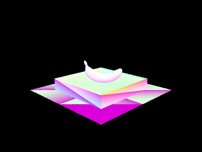
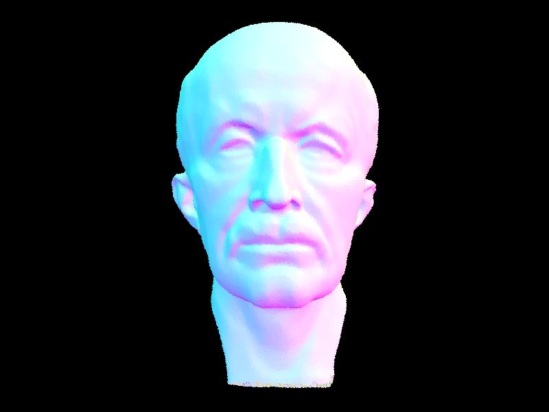
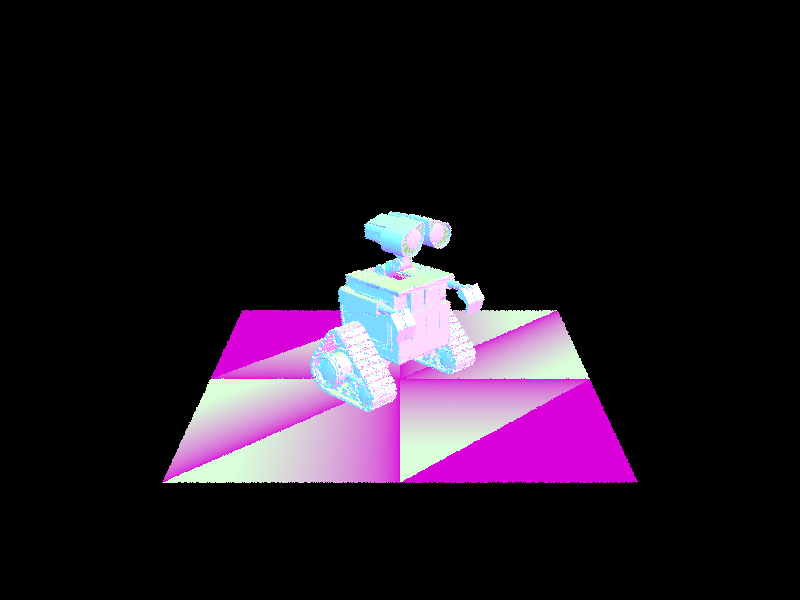
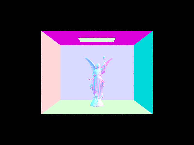
Here are some generated images with normal shading:

Part 2: Bounding Volume Hierarchy

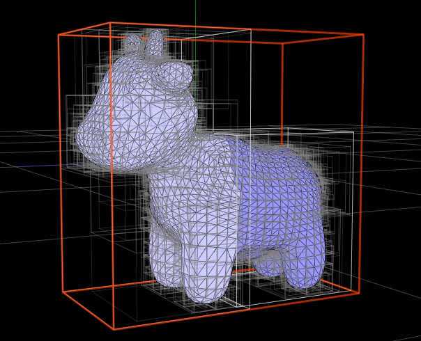
The BVH construction algorithm recursively partitions the set of primitives to create a hierarchical structure that accelerates ray-primitive intersection tests. It begins by computing a bounding box that encloses all primitives in the current subset. If the number of primitives is less than or equal to the maximum leaf size, the node becomes a leaf and stores the primitives directly. Otherwise, the algorithm proceeds to split the primitives into two groups, thereby creating two child nodes.

The heuristic for splitting is based on the spatial distribution of the primitives. Specifically, the algorithm chooses the axis along which the bounding box has the largest extent, ensuring that the split is made along the dimension where the primitives are most spread out. The splitting point is then chosen as the midpoint of the minimum and maximum bounds along this axis. Primitives are assigned to the left or right group based on whether the centroid of their bounding box lies below or above this midpoint. If the split happens to be unbalanced, a fallback to a median split is used to maintain a balanced tree structure. This strategy effectively reduces the overlap between bounding volumes and leads to efficient traversal during intersection tests.

The impact of BVH acceleration on rendering times is significant. Testing on scenes with moderately complex geometries, Planck's face rendering took roughly \(343.6477\) seconds without BVH acceleration, compared to just \(0.6870\) seconds with BVH. Additionally, the average number of ray intersection tests dropped from nearly \(27699.622246\) per ray without BVH to only \(31.174610\) with it. Similarly for the CBlucy scene rendering without the BVH took \(1008.6314\) seconds while rendering with BVH completed in just \(0.6267\) seconds accompanied by a similar drop in ray intersections per ray from \(79710.566331\) to \(29.172556\).

This reduction is primarily due to the hierarchical structure of the BVH, which reduces the average number of intersection tests from \(O(n)\) to approximately \(O(log n)\). These results illustrate how BVH acceleration scales well with increasing scene complexity, enabling more efficient rendering without compromising detail.

Here's also a picture of the BVH on a cow mesh:

Part 3: Direct Illumination

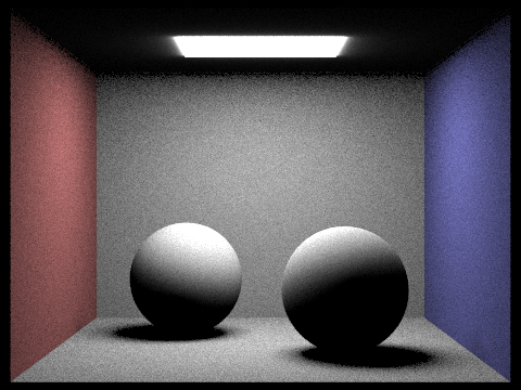
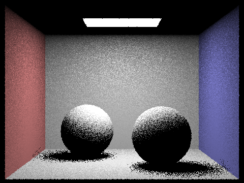
For direct lighting there are two main implementations: uniform hemisphere sampling, and importance sampling lights. Both implementations aim to compute direct lighting at an intersection point, but they differ in their sampling strategies.

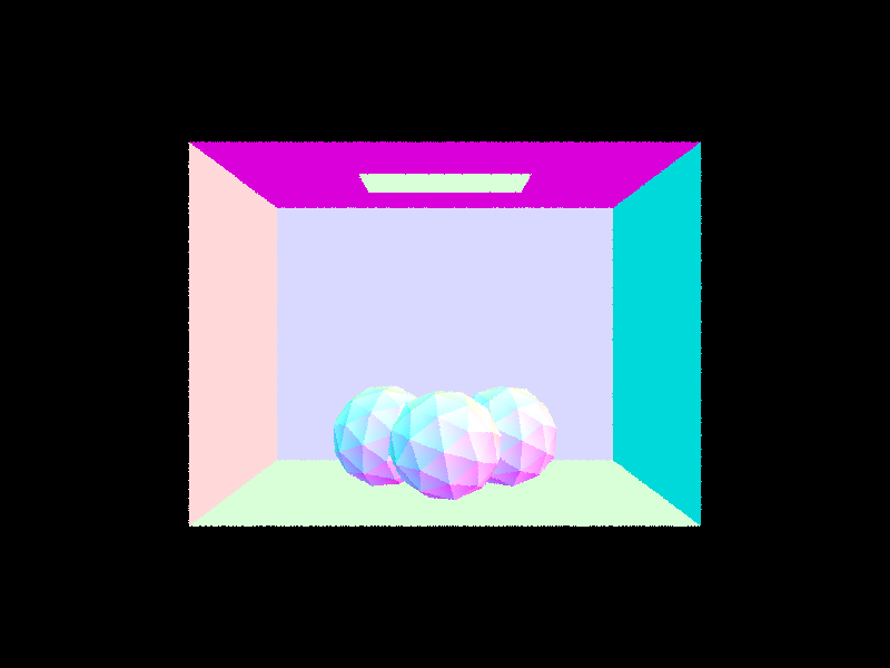
In the hemisphere sampling method, rays are uniformly distributed over the hemisphere above the surface. This approach gathers contributions by testing if these rays intersect any light-emitting surfaces and then scales the light's radiance by the cosine of the angle between the surface normal and the sample direction. Although this method is conceptually simple and provides a baseline, it tends to miss the directional characteristics of area lights resulting in less pronounced glow around the light sources, because it doesn't target the light sources directly.

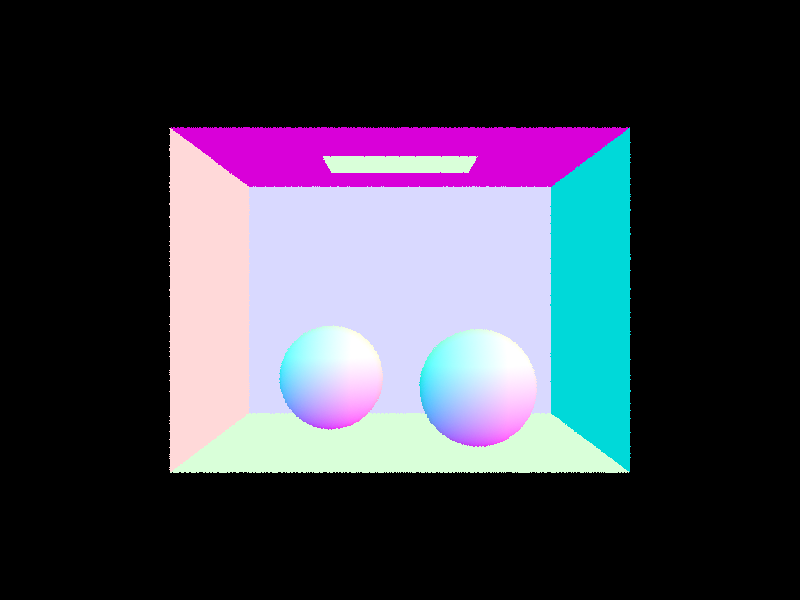
On the other hand, the importance sampling method focuses on sampling the light sources themselves rather than the entire hemisphere. This approach iterates over each light in the scene, sampling a direction based on the light's distribution and computing the corresponding contribution if the path is unobstructed. By carefully setting up shadow rays with a proper offset and limiting their travel to just before the light (using an epsilon value), this technique efficiently captures the direct lighting with reduced variance and noise. The importance sampling method is generally more robust, especially in scenes where the lighting is dominated by a few significant light sources, as it directly accounts for the light's spatial extent and directionality.

Clearly noise in the renders above goes down significantly when using importance sampling. The graininess just completely goes away. This demonstrates the effectiveness of the importance sampling technique in producing drastically higher render quality for the same number of samples. We reduce variance because we know where the lights are and thus the samples we are making are more "meaningful".

Here's also a picture of a dragon using importance sampling: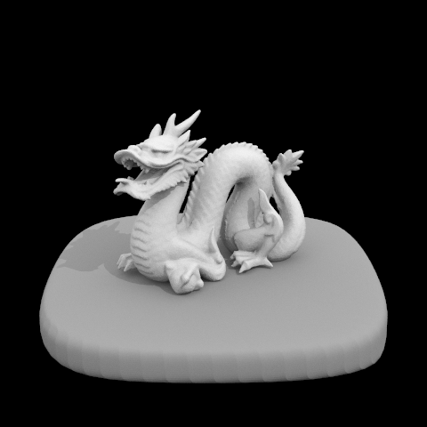 Now I compare the noise levels in soft shadows when rendering with 1, 4, 16, and 64 light rays (the -l flag) and with 1 sample per pixel (the -s flag) using light sampling, As seen above as the number of light rays increases, the noise in soft shadows decreases significantly. In the picture with -l 1, the soft shadows are very speckly and sharp, whereas the render using 64 light rays has very smooth soft shadows.

Part 4: Global Illumination

This function computes the radiance at a surface point by combining direct illumination (using one bounce of light) with additional indirect illumination from extra bounces. First, the function builds a coordinate system aligned with the surface normal to transform vectors between world and local space. It computes the hit point and the outgoing direction in local coordinates. Then it adds the one bounce radiance (direct light) calculated by another function. For the indirect component, it samples the BSDF to obtain a scattering direction and its probability density function (pdf). Note late we also implement a Russian roulette strategy (with a 70% continuation probability) is applied to probabilistically terminate paths while ensuring energy is conserved by dividing by the roulette probability. If the sample is accepted and the new ray (with reduced depth) intersects a light source or another surface, the function is recursively called to compute the radiance from that bounce. The indirect contribution, weighted by the BSDF, cosine term, and pdf, is then added to the overall radiance.

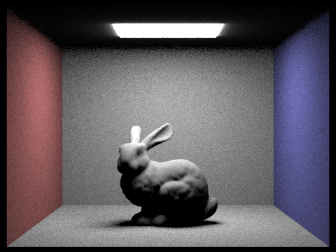
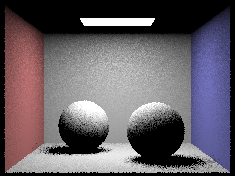
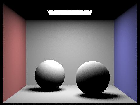
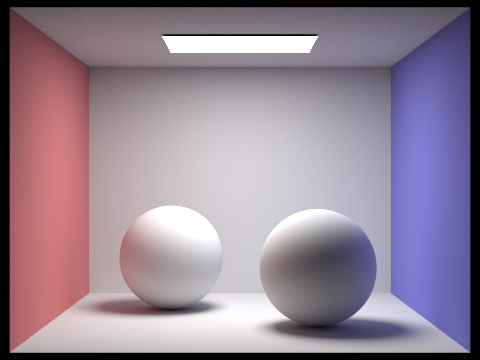
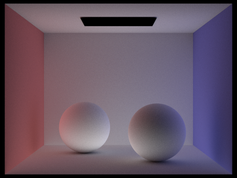
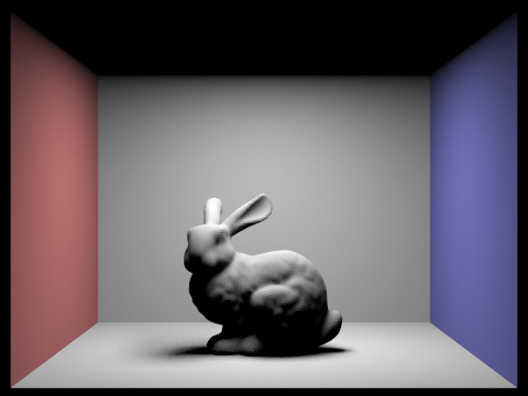
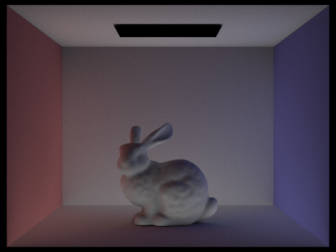
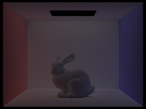
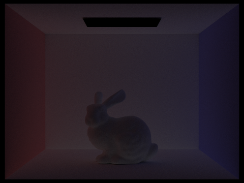
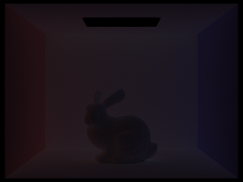
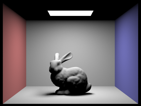
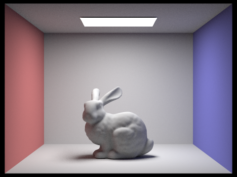
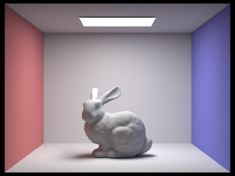
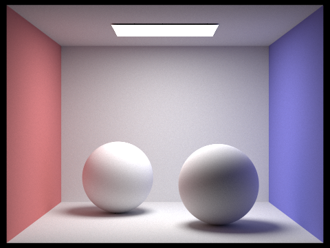
Here are some images rendered with global (direct and indirect) illumination using 1024 samples per pixel. Next we compare rendered views first with only direct illumination, then only indirect illumination using 1024 samples per pixel.

Now we render the mth bounce of light with max_ray_depth set to 0, 1, 2, 3, 4, and 5 (the -m flag), and isAccumBounces=false. At the 2nd and 3rd bounces, we start to see significant contributions to global illumination. The second bounce allows light that initially hit the floor or walls to reflect onto more occluded surfaces, such as the front of the bunny or the ceiling, areas that direct lighting may not reach. By the third bounce, light has had enough opportunities to scatter throughout the room, noticeably brightening shadowed regions and enhancing the overall soft, realistic appearance of the scene.

Compared to rasterization, which typically only simulates direct lighting and perhaps a single bounce via techniques like screen-space reflections, path tracing with multiple bounces captures much richer indirect lighting. This results in more natural color bleeding, softer shadows, and a better sense of depth. By around 2-3 bounces, most key surfaces in the room have been reached by light, so additional bounces beyond that offer diminishing returns in visual difference, though they continue to refine subtle lighting effects.

For comparison we have the accumulated bunny for m=0,1,2,3,4,5: For CBbunny.dae, we output the Russian Roulette (with continuation probability 0.6) rendering with max_ray_depth set to 0, 1, 2, 3, 4, and 100(the -m flag) using 1024 samples per pixel and -l 1. Using the bunny scene we compare rendered views with various sample-per-pixel rates, 1, 2, 4, 8, 16, 64, and 1024 using 4 light rays.

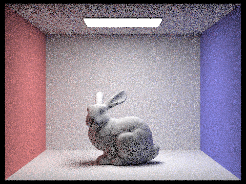
Part 5: Adaptive Sampling

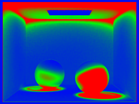
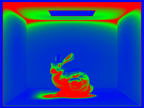
Adaptive sampling is a strategy designed to use computational resources more efficiently by varying the number of samples taken per pixel based on how quickly that pixel converges to a stable value. Instead of uniformly applying a high sample count to every pixel, we monitor the statistical variance of the samples in each pixel. For each pixel, we accumulate samples and calculate the running mean and standard deviation of the illuminance. Using these values, we compute a 95% confidence interval. When this margin of error becomes smaller than a set fraction of the mean (i.e., \(I\leq\)maxTolerance*\(\mu\)), we can be confident that the estimated value is close to the true value and stop further sampling for that pixel. In essence, adaptive sampling saves time and resources by allowing pixels that quickly reach a reliable estimate to stop sampling early, while pixels with higher variance continue to be sampled until they converge.

In our adaptive sampling implementation, we start by initializing accumulators for the total radiance, the sum of illuminance values (s1), and the sum of squared illuminance values (s2), along with counters for the total number of samples (n) and samples in the current batch (batch_count). For each pixel, we loop through the maximum allowed samples, generating camera rays and computing the radiance using our global illumination function. With each sample, we update s1 and s2 using the pixel's illuminance, and accumulate the radiance. Once we reach a full batch of samples (determined by samplesPerBatch), we calculate the mean illuminance and the variance from s1 and s2, then compute the confidence interval width I using the formula I = 1.96 * sqrt(variance) / sqrt(n). If this interval is within a threshold (maxTolerance times the mean), we determine that the pixel has converged and exit the loop early. Otherwise, we reset the batch counter and continue sampling until convergence or the maximum sample count is reached. Finally, we compute the average radiance for the pixel and update the output buffers accordingly.