CS184/284A Spring 2025 Homework 2 Write-Up

Link to webpage: hw2.html
Link to GitHub repository: https://github.com/cal-cs184-student/sp25-hw2-leooooo

Overview

In this project, we implemented the de Casteljau algorithm for evaluating Bezier curves and surfaces, area-weighted normals for Phong Shading, as well as fundamental mesh operations, such as edge flips, edge splits, and upsampling via Loop subdivision, using a halfedge mesh data structure. Successful implementation of these features is central to effective geometry processing in computer graphics. Through this project, I deepened my understanding of Bezier evaluation and became proficient with mesh traversal and manipulation using the halfedge structure. The results and screenshots in this write-up illustrate the variety of geometric objects and processing techniques achievable with these methods.

Section I: Bezier Curves and Surfaces

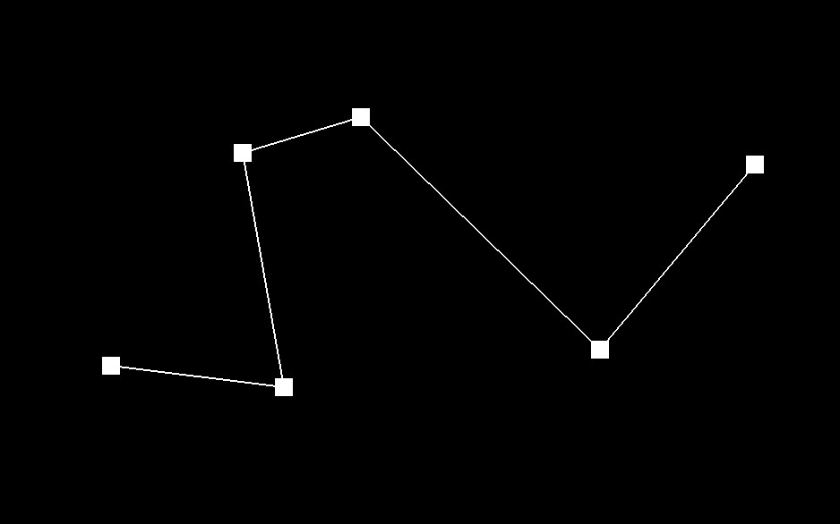
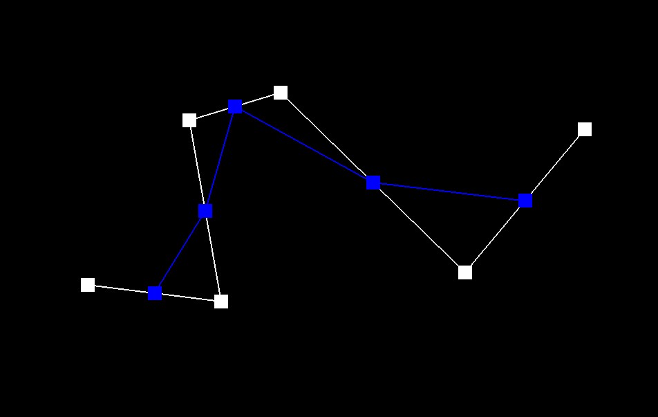
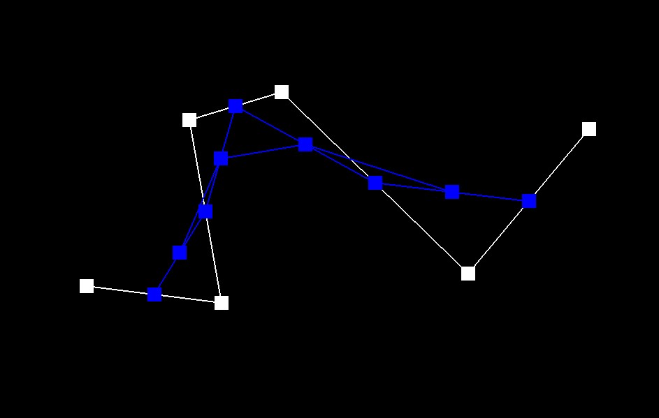
Part 1: Bezier curves with 1D de Casteljau subdivision

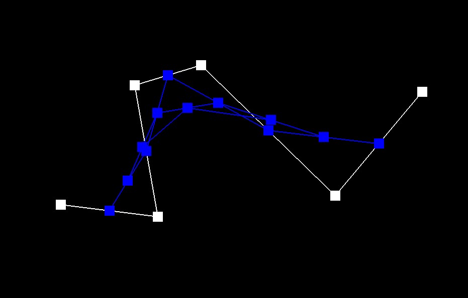
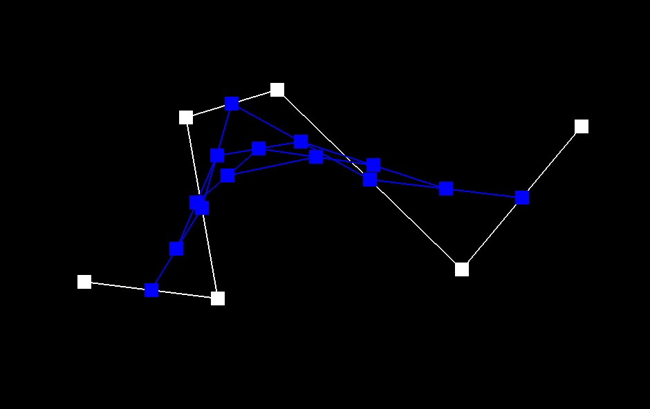
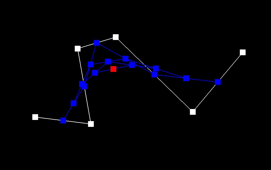
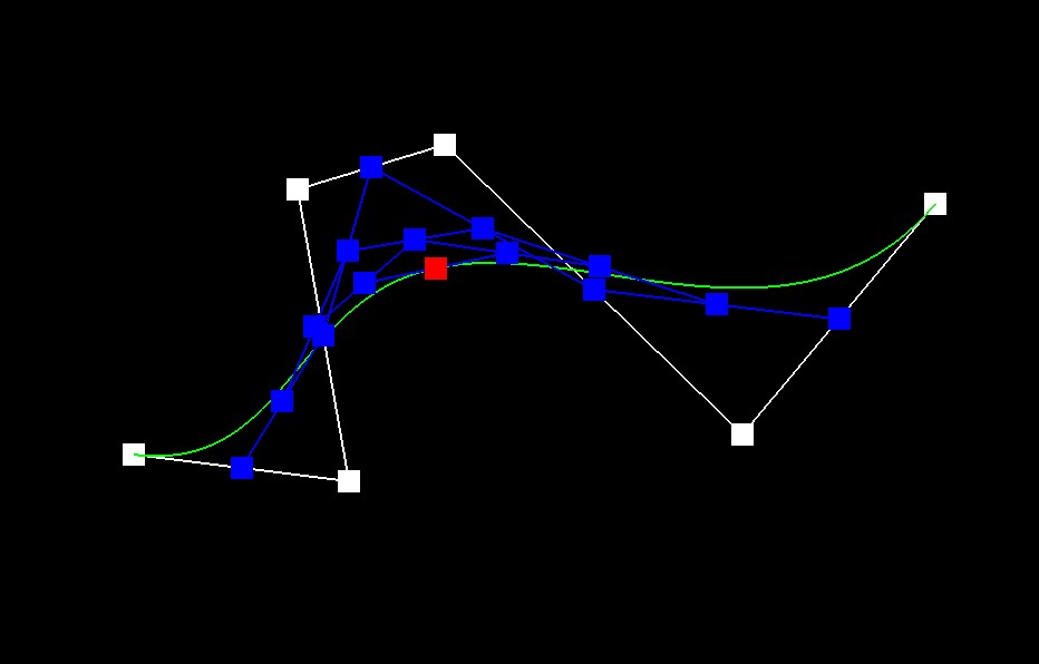
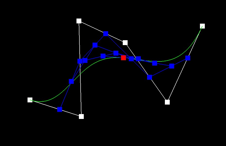
De Casteljau's algorithm is a recursive method for evaluating Bezier curves. Given a set of control points and a parameter \(0 \leq t \leq 1\) the algorithm repeatedly applies LERPs to adjacent points to generate new sets of points until only a single point remains. That final point is the point on the Bezier curve at the parameter \(t\). For implementation we have an evaluate step function that takes a vector of control points (possibly an intermediate list) and applies the LERP between each pair of points returning a new vector of intermediate points. When there is only 1 point left we return it.

Here are screenshots of each step / level of the evaluation from the original control points down to the final evaluated point and associated curve.

Here is a slightly different Bezier curve by moving the original control points around and modifying the parameter \(t\).

Part 2: Bezier surfaces with separable 1D de Casteljau

De Casteljau's algorithm extends naturally from curves to surfaces by applying the algorithm in two separable stages. First, each row of control points (from a 2D grid) forms a Bezier curve. First, the algorithm is applied along the \(u\) direction using the 1D de Casteljau process to each row to compute an intermediate point for that row. The intermediate points from each row now form a new set of control points along the \(v\) direction. Then the De Casteljau algorithm is applied to these points using the parameter \(v\) to compute the final point on the surface. For the implementation, I implemented a function similar to the 1D case, evaluateStep, which interpolates between adjacent points. Using evaluateStep, the evaluate1D function recursively computes a single point from a vector of points. For the surface evaluation, the evaluate function first computes an intermediate point for each row using evaluate1D with parameter \(u\). These intermediate points are then passed to another call of evaluate1D with parameter \(v\) to obtain the final Bezier surface point.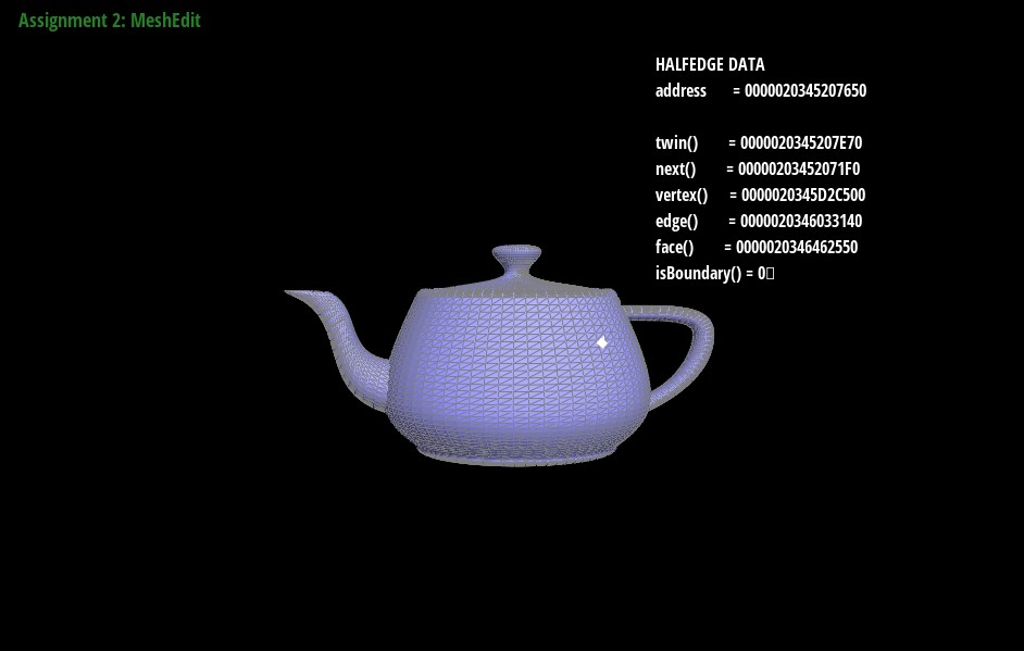

Section II: Triangle Meshes and Half-Edge Data Structure

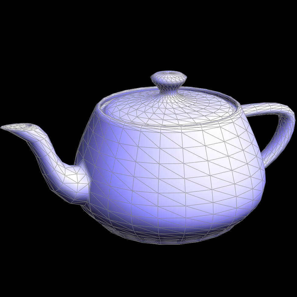
Part 3: Area-weighted vertex normals

The implementation computes the area-weighted normal by iterating over the neighboring ring of triangles around the vertex. For each adjacent triangle, it calculates the face normal using the cross product of two edge vectors and weights it by the triangle's area. The weighted normals are summed, and the final normal is obtained by normalizing this sum. This ensures that larger triangles have a greater influence, leading to a smoother normal representation.

Part 4: Edge flip

Implementing the edge-flip operation required careful pointer manipulation to ensure proper reassignments. I began by sketching the halfedge connectivity on paper, labeling each relevant element and mapping out the necessary changes. This visualization helped clarify how to reassign halfedges, vertices, and faces while maintaining a valid mesh structure. Before proceeding, I checked that the target edge was not on the boundary. Using a halfedge traversal similar to the function printNeighbourPositions, I created temporary variables for all affected elements and then methodically reassigned pointers based on my initial sketches. By following this structured approach, I avoided major debugging issues.

Part 5: Edge split

For implementing edge splitting, I took a similar, careful, and somewhat tedious approach as in Task 4. I started by drawing out all the halfedges, edges, and vertices involved in the operation. Then, I visualized the desired structure of the new triangles after the split and accounted for the new vertex and edges that needed to be added. By systematically tracking all the necessary pointer updates, I ensured that the mesh remained well-formed and consistent. Here is a picture of my diagram: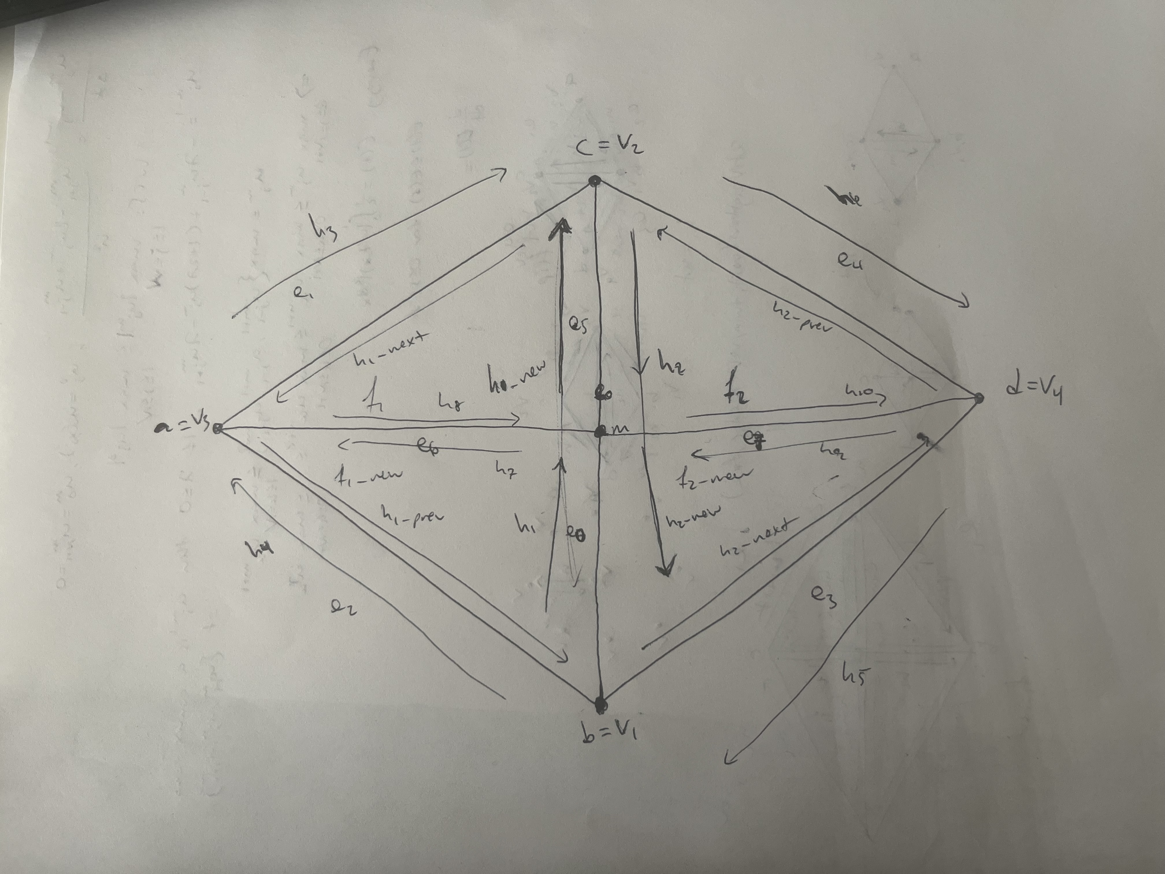

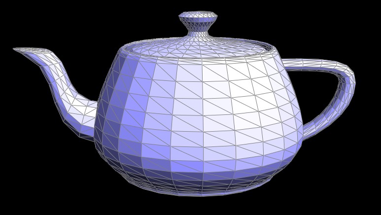
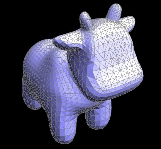
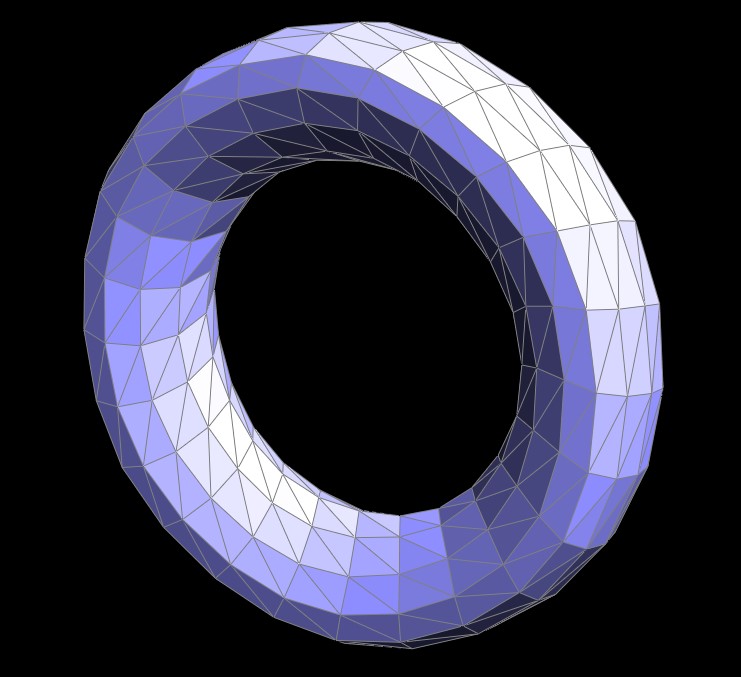
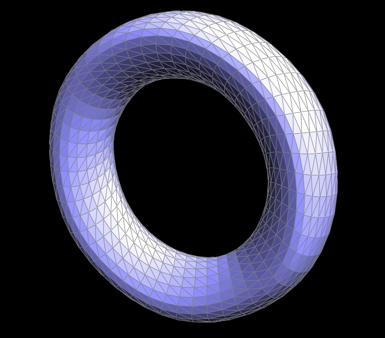
Part 6: Loop subdivision for mesh upsampling

To implement Loop subdivision, I followed several key steps. First, I computed new positions for all vertices in the input mesh using the Loop subdivision rule. This rule assigns weights to neighboring vertices so that each vertex's new position is a weighted average of its original position and those of its neighbors. I stored these computed positions in the temporary newPosition field and marked each original vertex as “old” by setting its isNew flag accordingly. Next, I computed the updated positions for the new vertices that will be inserted at edge midpoints. The rule for these “odd” vertices is based on a weighted average of the two vertices forming the edge and the two vertices opposite the edge in the adjacent triangles. I stored the result in each edge's temporary newPosition field. After the vertex and edge positions were computed, I split all the edges of the original mesh. To avoid an infinite loop from continuously splitting new edges, I ensured that only edges from the original mesh were processed by adding isNew flags to my task5. During each split, I transferred the precomputed edge position to the new vertex and updated the isNew flag on the resulting edges appropriately. Finally, to regularize the mesh topology, I iterated over the new edges and flipped any edge that connected an original vertex to a new vertex. This flip ensures that the resulting mesh has the desired structure. In the last step, I copied the new positions stored in the temporary fields into the actual vertex positions of the mesh

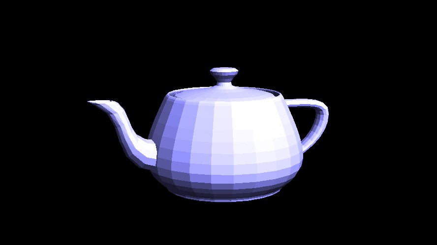
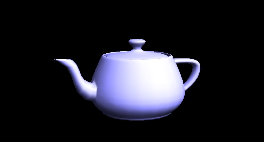
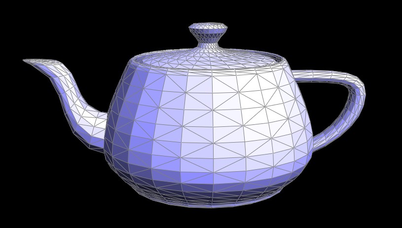
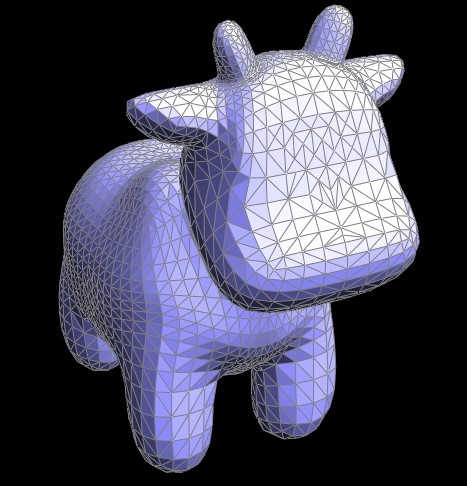
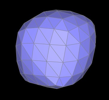
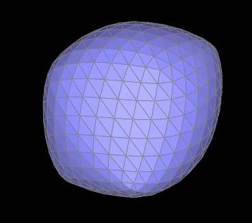
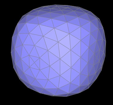
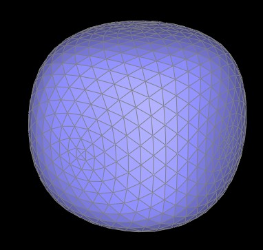
After applying Loop subdivision, I noticed that the mesh's sharp features tend to persist to some extent because the vertex updates use weighted averages that still “remember” the original crease. In my tests, the lower right and lower left regions of the unsplit mesh retained noticeably sharper corners and edges. However, when I pre-split those edges before subdivision, additional vertices were inserted along the crease, which allowed the averaging process to blend the positions more evenly. This resulted in smoother, more gradual transitions at those formerly sharp features. The screenshots below clearly show that the mesh without pre-splitting appears crisper along its edges, while the pre-split version exhibits a softer, more rounded appearance.

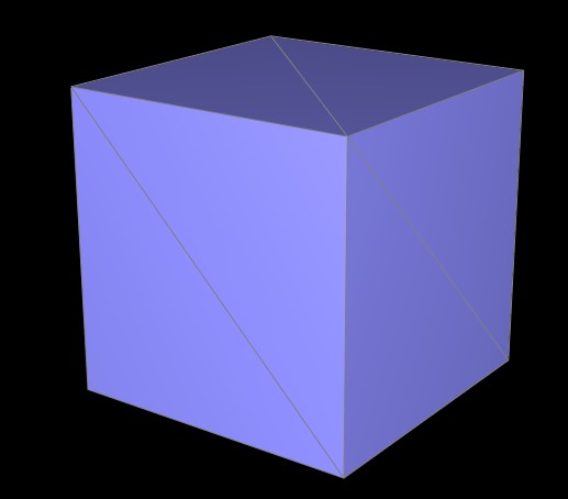
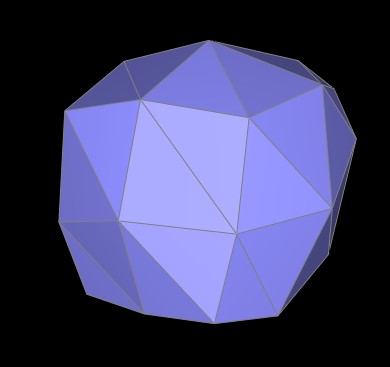
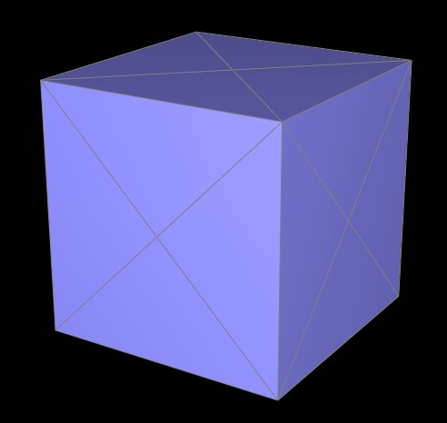
Below is an example demonstrating how a cube, when subjected to repeated loop subdivision without pre-processing, gradually becomes asymmetric. This occurs due to the presence of irregular edge configurations that introduce extraordinary vertices, disrupting the symmetry of the original shape. A uniformly preprocessed cube, using strategic splits, maintains symmetry during subdivision by preventing extraordinary vertices. This highlights how initial mesh topology influences subdivision outcomes, without preprocessing asymmetry grows over iterations while a well-structured mesh preserves the cube's form.

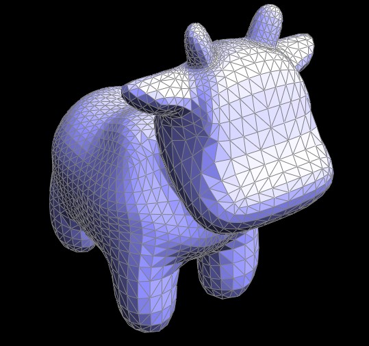
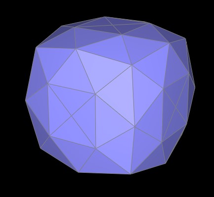
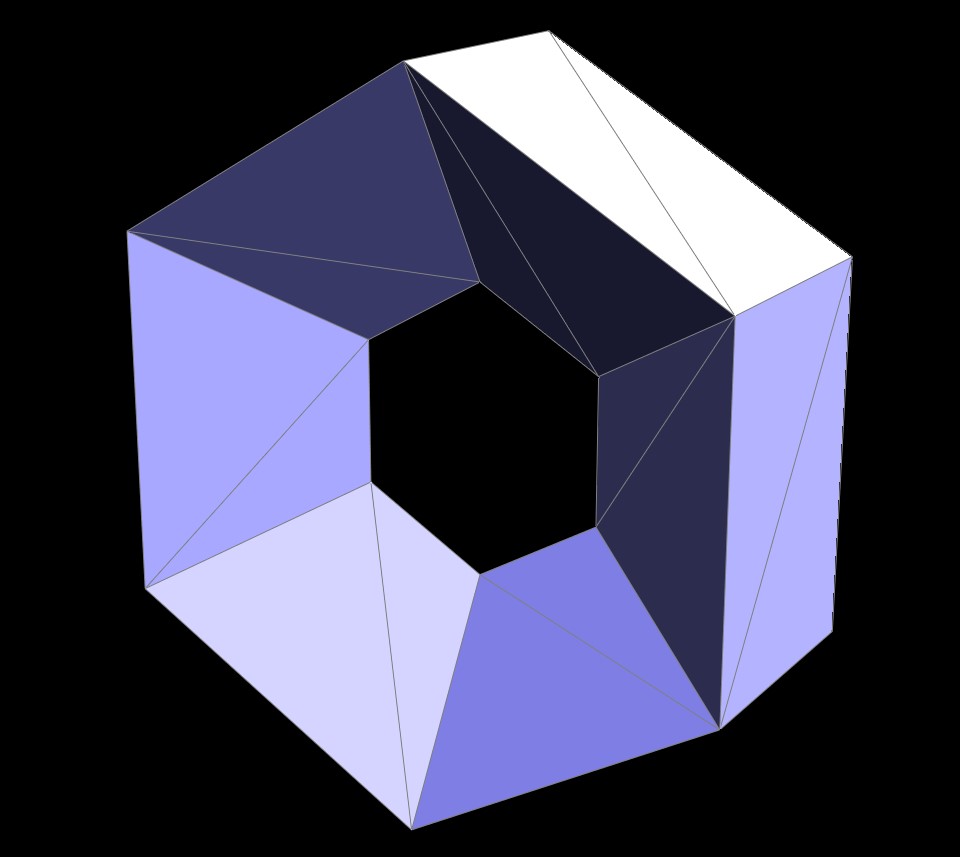
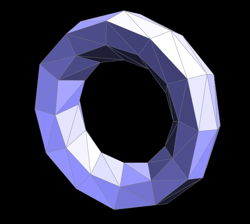
Here are some extra images of upsampling: